
SLOPE
SLOPE assigns larger weights to larger coefficient magnitudes. Here denotes the th largest absolute value. Its corners can encourage equal magnitudes, including coefficients with opposite signs. Supply exactly one finite, nonnegative, nonincreasing weight per coefficient; the weights already include the penalty strength.
Constraint region
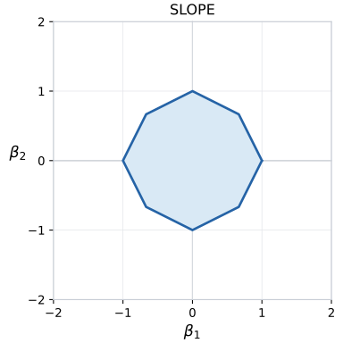
: . See the plot conventions for the fixed budget and coefficient scale.
Use the penalty
use ;
Equal weights recover lasso. Repeated weights and trailing zeros are valid; all-zero weights give no penalty. Use proximal gradient or the hybrid solver with Gaussian or binomial datafits. The SLOPE fitting guide explains magnitude clusters and advanced controls.
API: shrinkage::Slope.